Computer Vision-based Fluid-Structure Interaction Tracking Software

Project Scope

Ionic polymer-metal composites (IPMCs) are a type of electroactive polymer typically used in soft-robotic applications. The unique two-way transduction property of IPMCs allows for both actuation and sensing, which, in conjunction with its ability to be used in aqueous environments, can be used for various underwater applications. For this study, we aim to use the IPMC’ s unique sensing capabilities as an underwater flow sensor, capable of measuring the flow field of the surrounding environment. This approach is dependent on signal characterization of the acquired voltage response and the fluid dynamics phenomenon of Kármán vortex streets. The latter requires the sensor to detect the frequency of vortex shedding from either the sensor itself or from an obstructing object positioned before the IPMC sensor. The project was split into three major goals:

1. Capture and track the relative velocity of IPMC sensor using imaging and image process techniques.Confirm this value with our known value, and calculate expected vortex shedding frequency with this velocity.
2. Capture and and measure the tip displacement of the IPMC sensor during travel using imaging and image process techniques, and compare to acquired voltage data from the sensor.
3. Capture and display shed vortices from the experiment.

Ionic Polymer-Metal Composites: An Overview

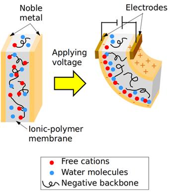
IPMCs are unique electroactive polymers in that they exhibit both electromechanical (electrical to mechanical) and mechanoelectrical (mechanical to electrical) transduction, like that of piezoelectric materials, and are constructed from flexible polymers that can sustain large deformations and strains. The core structure of an IPMC is an ionomeric-polymer (ionomer), which consists of strong ionic groups attached to a charge-neutral polymer backbone. With this ionomer structure, the IPMC is formed by compositing an electrode material, typically a noble metal (such as platinum, gold, palladium, or silver), onto the surface of a thin ionomer membrane. This process forms the final material, a combined structure of an ionomer and metal electrodes, forming an ionic polymer-metal composite.

The choice of backbone ionomer, electrode material, mobile ion species, solvent, and hydration level all have an immense impact on the behavior and performance of IPMC materials, demonstrating their highly complex nature.

Regarding IPMCs as a sensor, induced deformation is believed to cause a redistribution of cations within the porous network due to mobility in the solvent, in addition to the anion-clusters deforming with the material such that the clusters form effective dipoles which induce a detectable signal along the electrodes, often within the millivolt range. The work presented herein will be focused on this aspect of IPMC physics.

Principles of Flow Sensing

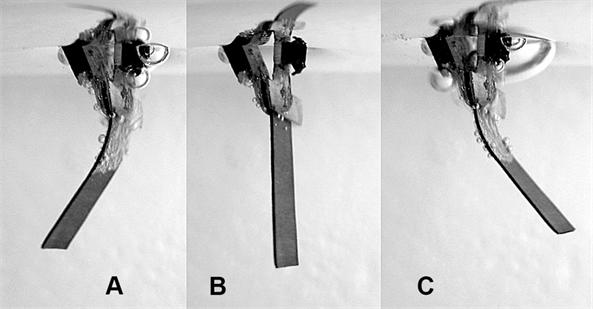
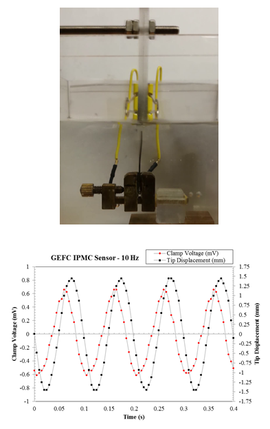
One of the more prominent uses of IPMC sensors in underwater applications has been in the development of IPMC-based flow sensor devices. There have been two approaches in this endeavor, one of which involves interpreting the characteristic response directly, and the other requiring additional signal processing within the frequency domain. The former is dependent relating the acquired voltage response directly to the environmental causes of displacement surrounding the IPMC. The figure below is a still-frame of an oscillating IPMC due to a shaker at 10 Hz.

Experimental Setup

Equipment

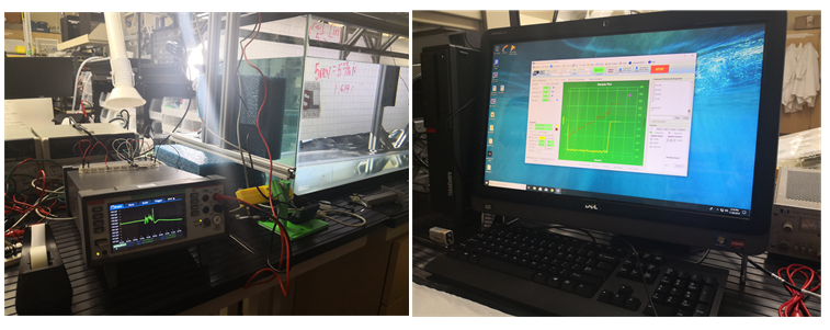
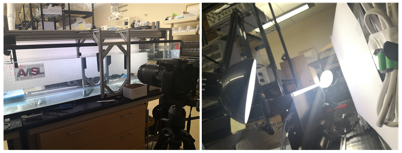
Experiments were conducted within an 85 gal aquarium with the IPMC sensor mounted to an inverted linear belt slide system (MacronDynamics MSA-M6S) driven by an stepper motor (Applied Motion Products SSM23IP-4EG). The motor software was programmed to run at 200 rps, traveling at 150 mm/rev (300 mm/s). Voltage readings were acquired directly using a Keithley 6510 DAQ.

Camera Configuration

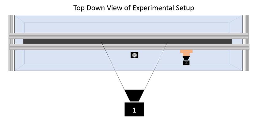
Camera 1: Velocity (Canon EOS Rebel SL1)

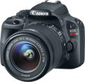
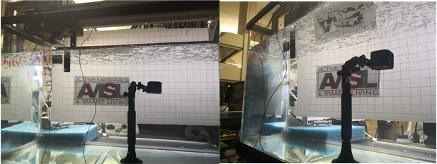
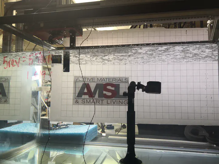
Fixed directly facing the side wall of the aquarium, camera 1 will be capturing the travel of the sensor mount. The camera is fitted with the stock 18-55mm Canon lens. Video was captured at 1080p, 30 fps. The far-side of the aquarium is fitted with a 1 inch grid poster that will be used when determining the calibration factor of the footage. Various light-sources were set behind the background image in order to produce a backlit, silhouette-esq footage of the sensor mount traveling.

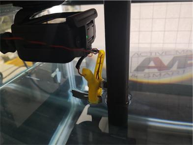
Camera 2: Tip Deflection (OSMO Action)

Camera 2 was mounted directly to the carriage to travel alongside the sensor, directly observing sensor deformation from an above view. Camera 2 will be used to relate the dynamic tip displacement of the IPMC to the acquired voltage response. Camera 2 captured high speed footage at 1080p, 240 fps, ideally to capture the nuance in the deformation.

Camera 3: Particle Tracking (GoPro Hero4 Session)

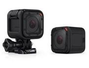
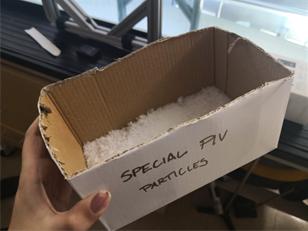
Camera 3 was placed at a fixed location on the floor of the aquarium where it was used to capture the life cycle of the shed vortices from the carriage/bluff body. The camera was set to capture footage at 1080p, 30 fps. In addition, to better visualize the vortices, packing foam was shredding into pieces, ultimately functioning as tracking particles which assisted in image processing the flow trends on the surface of the water.

Implementing Mathematica

Velocity Tracking

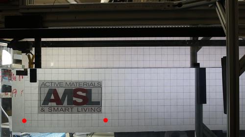
In this section, Mathematica was implemented to detect the velocity of a discrete binarized section of the sensor carriage mount. The found velocity can then be used in calculating the expected frequency of vortex shedding and can be used to verify the set velocity from the provided linear belt slide software. An assumption is made that the carriage, clamp, and IPMC sensor are traveling as a single body, and thus share the same velocity. Prior to analysis, the captured experimental video was exported as a series of .png images through an external video editing software, which was then imported into Mathematica in the following cells. The images must be resized due to the large quantity. The spatial calibration factor was determined using the 1" grid background, which is highlighted in the first image shown.

(* Setting Directory and Accessing Images *)
SetDirectory["dir"]; 
(* Change file directory to file containing images *)
images = FileNames["*.png"];
count = 1;
Do[imagevar[count++] = Import[image], {image, images}];

(* Storing and Resizing Images *)
Table[imagevar[i], {i, 1, 60}];
sideimgs = Map[ImageResize[#, 500] &, %];

(* Using Background for Spatial Calibration - each square was 1", 1 \
ft total *)
coords = {{215.`, 35.`}, {49.`, 34.`}};
HighlightImage[sideimgs[[1]], {coords[[1]], coords[[2]]}]

(* Finding Calibration Factor and Labeling Important Variables*)
distperpixel = 304.8/EuclideanDistance[coords[[1]], coords[[2]]];
fps = 30;
dt = 1/fps;
tmax = Length[sideimgs]*dt;

A mask was applied to isolate a specific region of capture that will be used for simplifying the binarization of the moving carriage. With the mask applied, the series of images were then color separated into CMYK color channels. The yellow channel, which best isolated the color of the clamp, was used to easily identify the moving carriage using a threshold binarization. The ComponentMeasurements function was then applied to determine the centroid of the binarized component within each frame. The “centroids” variable was specifically used for velocity measurement, while “centroid” was used for highlighting the carriage in the tracking animation.

(* Applying mask to focus on specific region *)
mask = "maskimg";
binimgs = sideimgs*mask;

(* Color Separating and Binarizing Yellow Channel *)
binimgs = Map[ColorSeparate[#, "CMYK"][[3]] &, binimgs];
Map[DeleteSmallComponents[Binarize[#, 0.7]] &, binimgs];
centroid = Map[ComponentMeasurements[#, "Centroid"] &, %][[All, 1, 2]]; (* Centroid for Highlight Image *)
centroids = Map[ComponentMeasurements[#, "Centroid"] &, %%][[All, 1, 2, 1]]; (* Centroid for Velocity Component *)

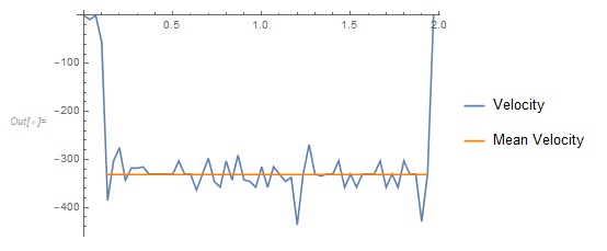
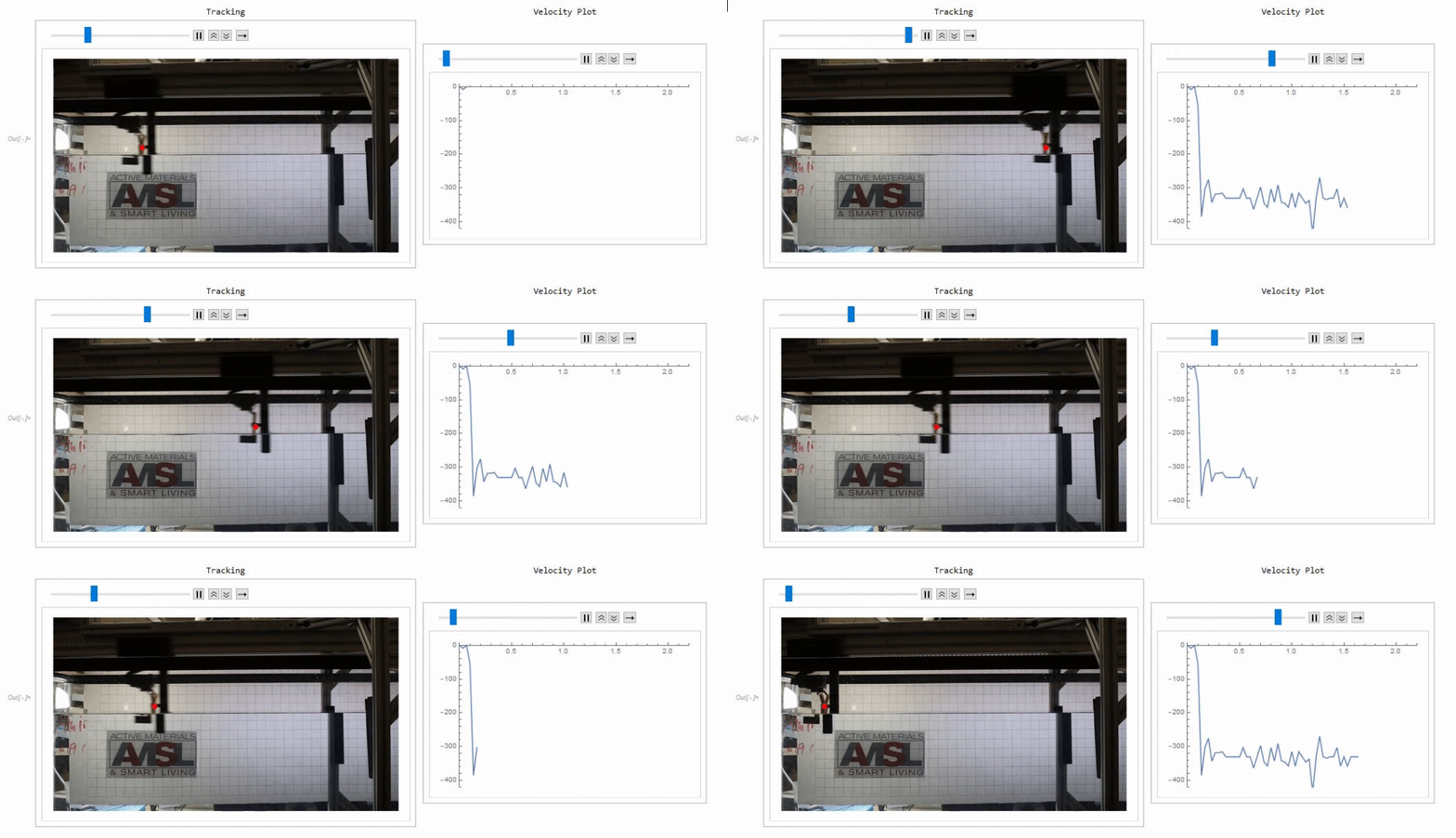
A list of velocities were then established by determining distance travel in successive frames and then by subsequently dividing the time step and and multiplying by the calibration factor. A “0” value was appended to the velocity list to account for the carriage exiting the FOV at the final frame. A mean velocity was then calculated by partitioning a stable region of velocities. The results were then plotted using ListLinePlot.

(* Velocity and Time *)
velo = Table[-distperpixel*(centroids[[i + 1]] - centroids[[i]])/
     dt, {i, 1, Length[centroids] - 1}];
time = Range[0, tmax, dt];
velo = Table[{time[[i]], velo[[i]]}, {i, 1, Length[velo]}];
velo = Append[velo, {59/30, 0}]; (* Adding 0 to end *)

(* Mean Velocity Line *)
peakvel = Table[{time[[i]], Mean[peakvelo]}, {i, 5, Length[velo] - 1}];

(* Plotting *) 
(* Velocity and Time *)
velo = Table[-distperpixel*(centroids[[i + 1]] - centroids[[i]])/
     dt, {i, 1, Length[centroids] - 1}];
time = Range[0, tmax, dt];
velo = Table[{time[[i]], velo[[i]]}, {i, 1, Length[velo]}];
velo = Append[velo, {59/30, 0}]; (* Adding 0 to end *)

(* Mean Velocity Line *)
peakvel = Table[{time[[i]], Mean[peakvelo]}, {i, 5, Length[velo] - 1}];

(* Plotting *) 
Show[{ListLinePlot[velo, PlotLegends -> {"Velocity"}], 
  ListLinePlot[peakvel, PlotStyle -> Orange, 
   PlotLegends -> {"Mean Velocity"}]}]
peakvelo = {-383.27456575836163`, -301.14430166728414`, \
-261.3235675625189`, -368.34179046907514`, -313.5882810750235`, \
-303.6330975488312`, -313.5882810750235`, -328.52105636430997`, \
-328.52105636430997`, -301.14430166728414`, -355.8978110613358`, \
-328.52105636430997`, -301.14430166728414`, -316.7881614941556`, \
-328.52105636430997`, -373.10605687089503`, -310.87825889289326`, \
-313.31174819929595`, -343.73036452932394`, -355.621278185609`, \
-301.42083454301087`, -328.52105636430997`, -301.57885332914157`, \
-340.2539512344643`, -343.73036452932394`, -340.6885028963218`, \
-328.52105636430997`, -355.8978110613358`, -328.52105636430997`, \
-328.52105636430997`, -312.09500354609384`, -328.52105636430997`, \
-432.55272421301`, -260.4702661174146`, -359.808776018056`, \
-332.43202132102704`, -328.52105636430997`, -328.52105636430997`, \
-328.52105636430997`, -328.52105636430997`, -328.52105636430997`, \
-328.52105636430997`, -355.8978110613358`, -328.52105636430997`, \
-328.52105636430997`, -301.14430166728414`, -355.8978110613358`, \
-328.52105636430997`, -328.52105636430997`, -328.52105636430997`, \
-328.52105636430997`, -328.52105636430997`, -328.52105636430997`, \
-410.65132045538746`, -355.8978110613358`};
Mean[peakvelo]

(* Animating Plot *)
animvelo = Table[velo[[1 ;; i]], {i, 1, Length[velo]}];
animpeakvel = Table[peakvel[[1 ;; i]], {i, 1, Length[peakvel]}];
Grid[{{"Tracking", 
   "Velocity Plot"}, {ListAnimate[
    Table[HighlightImage[sideimgs[[i]], centroid[[i]]], {i, 1, 
      Length[sideimgs]}], 30], 
   ListAnimate[
    Table[ListLinePlot[animvelo[[i]], 
      PlotRange -> {{0, 2.2}, {-420, 0}}], {i, 1, Length[animvelo], 
      1}], 30]}}]

IPMC Displacement Tracking

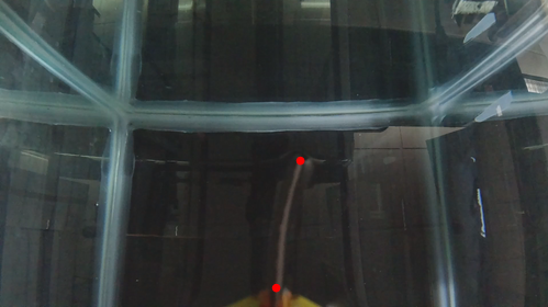
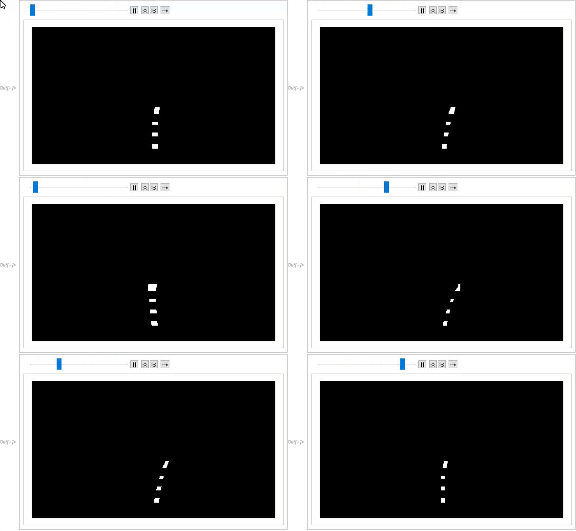
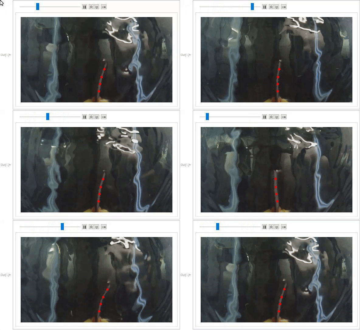
The following section of code is used to track IPMC deformation during travel. Similar to the first portion of code, images of gathered experimental footage were imported and resized for data management. Prior to binarization, a mask was applied to each frame to isolate the region of interest. Due to difficulty in binarization, a specific range of frames were chosen where the binarization was found to be the most stable. During binarization, a Sobel edge detection kernel was applied to increase accuracy of binarization by detecting the edge of the rectangular IPMC. A second mask was then applied to segment the IPMC into four sections for tracking curvature. There was difficulty in binarizing this set of footage due to the reflection of the water and almost near transparency of the IPMC. It may be useful to attempt to make the points of interest more prominent during experimental imaging for better clarity and accuracy during binarization. The ComponentMeasurement feature was then used to determine the centroids of each segmented section of the IPMC during travel.

(* Setting Directory *)
SetDirectory[
  "C:\\Users\\Nazanin\\Desktop\\Image Processing Project\\For \
Mathematica\\Tip Deflection\\"]; (* Change file directory to file \
containing images *)
images = FileNames["*.png"];
count = 1;
Do[imagevar[count++] = Import[image], {image, images}];

(* Storing and Resizing *)
Table[imagevar[i], {i, 1, 1164}];
topimgs = Map[ImageResize[#, 500] &, %];

mask1 = "mask1.jpg"; (* The first mask is applied for simplifying the initial binarization \
*)
mask2 = "mask2.jpg"; (* The second mask is applied to create 4 separate components which \
we will be tracking *)

(* Binarizing *)
Components = 
  mask2*Table[
    Closing[DeleteSmallComponents[
      EdgeDetect[Binarize[mask1*topimgs[[i]], .2], 
       Method -> "Sobel"]], 7], {i, 190, 500, 11}];
ListAnimate[Components]

(* Finding the centroids *)
centroids = 
  Table[ComponentMeasurements[Components[[i]], "Centroid"], {i, 1, 
    Length[Components]}];

The centroids were then mapped onto the footage of the IPMC for visual confirmation. Spatial calibration was then conducted using the length of the IPMC, which was known to be 30 mm from clamp to tip.

(* Grabbing images of just the frames of footage used *)
mapimgs = Table[topimgs[[i]], {i, 190, 500, 11}];
ListAnimate[
 Table[HighlightImage[mapimgs[[i]], centroids[[i, All, 2]]], {i, 1, 
   Length[mapimgs]}]]

(* Spatial Calibration - IPMC from clamp to tip was 30 mm *)
coords = {{273.`, 134.`}, {251.`, 18.`}};
HighlightImage[topimgs[[1]], {coords[[1]], coords[[2]]}]

(* Finding Calibration Factor and Labeling Important Variables*)
distperpixel = 
  30/EuclideanDistance[coords[[1]], coords[[2]]]; (* mm/px *)
fps = 240;
dt = 1/fps; (* Actual time step *)
dt2 = 11/fps; (* Samping gap from binarization step *)
t0 = 190*dt;(* initial time - starting frame*)
tf = 500*dt ;(* final time - ending frame *)
time = Range[0, (tf - t0), dt2] // N; (* Time range was approx 1.3 seconds *)

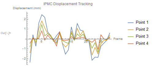
Displacement was calculated by determining the distance traveled by the centroid of successive frames. The centroid of each component was then plotted which reveals the effects of curvature, as the furthest points from the clamp have the highest amplitude. This displacement plot was also compared to the voltage response acquired from the IPMC directly using a data acquisition device. These two plots show very similar trends.

(* Displacement between component centroids per frame *)
Displacement = 
  Table[distperpixel*(centroids[[i + 1, All, 2]] - 
      centroids[[i, All, 2]]), {i, 1, Length[centroids] - 1}];

(* Plot of All Centroid Displacement *)
ListLinePlot[{Displacement[[All, 1, 1]], Displacement[[All, 2, 1]], 
  Displacement[[All, 3, 1]], Displacement[[All, 4, 1]]}, 
 PlotLegends -> {"Point 1", "Point 2", "Point 3", "Point 4"}, 
 PlotLabel -> "IPMC Displacement Tracking", 
 AxesLabel -> {"Frame", "Displacement (mm)"}]

(* Comparing to Voltage Response *)
s = Import[
   "C:\\Users\\Nazanin\\Desktop\\Image Processing Project\\11262019 \
Data\\Tip Deflection Data.xlsx"];
V = Table[{s[[1, i, 1]], (s[[1, i, 2]] - 0.00020)/0.00006}, {i, 1, 
    63}]; (* Normalizing Data *)
VoltagePlot = 
  ListLinePlot[V, PlotLabel -> "IPMC Voltage Response", 
   AxesLabel -> {"Time (s)", "Voltage"}, GridLines -> Automatic];

(* Attaching Relative Time to Max Displacement Data *)
X = Table[{time[[i]], Displacement[[i, 1, 1]]}, {i, 1, 
    Length[Displacement]}];
DisplacementPlot = 
  ListLinePlot[X, PlotLabel -> "IPMC Max Displacement", 
   AxesLabel -> {"Time (s)", "Displacement (mm)"}, 
   GridLines -> Automatic];
Grid[{{Show[VoltagePlot, ImageSize -> Medium], 
   Show[DisplacementPlot, ImageSize -> Medium]}}]

Particle Tracking

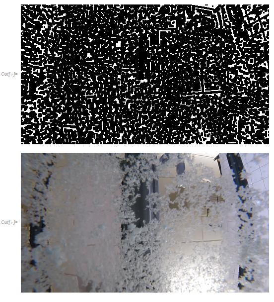
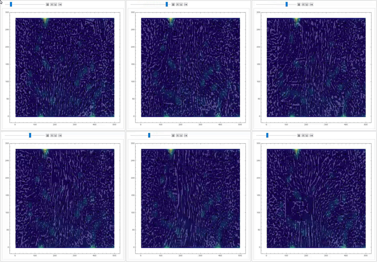
In this section, pseudo-PIV images were obtained to show flow patterns over time at a fixed location. Experimental images were imported and resized for data management. A local adaptive binarize was used in order to identify particles. The experiment setup created limitations in isolating particles during binarization and thus environmental objects are seen in binarized images. This will in turn affect the accuracy of flow pattern analysis. Having particles that are dissimilar to the environment can potentially allow for better tracking and flow pattern analysis.

(* Setting Location and Grabbing Files *)
SetDirectory[
  "C:\\Users\\Nazanin\\Desktop\\Image Processing Project\\For \
Mathematica\\Underwater\\"]; (* Change file directory to file \
containing images *)
images = FileNames["*.png"];
count = 1;
Do[imagevar[count++] = Import[image], {image, images}];

(* Storing Files and Resizing *)
Table[imagevar[i], {i, 1, 129}];
pivimgs = Map[ImageResize[#, 500] &, %];

(* Binarization *)
pivframes = 
  Table[Erosion[Opening[LocalAdaptiveBinarize[pivimgs[[i]], 4], 1], 
    1], {i, 20, 65, 1}];
pivframes[[1]]
pivimgs[[20]]
Transpose[ImagePartition[#, 25] & /@ pivframes, {3, 1, 2}];

An example of partitioning a frame to determine displacements of each section of a single image. An image correlate was used to determine these displacement vectors. Once these displacement vectors were found an animation was made of the binarized images with an overlay of the displacement vectors.

(* Example: Partitioning to 25 Boxes *)
GraphicsGrid[ImagePartition[pivframes[[1]], 25]] 
ColorNegate@
     ImageAdjust@
      Image[ImageCorrelate[#[[2]], #[[1]], 
        EuclideanDistance]] & /@ # & /@ %%(*calculate \
cross-correlations*)
ComponentMeasurements[Binarize[#, 0.9], "Centroid"][[1, 2]] - {32, 
       32} & /@ # & /@ %; (*get displacements*)

Final code below for determining the flow field. This code was found in Lecture 23 of ME 695.

Module[{imgs = pivframes}, 
 Module[{divisions = 25, windowsize, windowcenters, disps, 
   imgdims = ImageDimensions[imgs[[1]]], selects},
  windowsize = imgdims/divisions;
  windowcenters = 
   Table[Table[{j*windowsize[[1]] - windowsize[[1]]/2, 
      i*windowsize[[2]] - windowsize[[2]]/2}, {j, divisions}], {i, 
     divisions}];
  disps = 
   ComponentMeasurements[
          Binarize[
           ColorNegate@
            ImageAdjust@
             ImageCorrelate[#[[2]], #[[1]], EuclideanDistance], 0.9], 
          "Centroid"][[1, 2]] - windowsize/2 & /@ # & /@ 
    Transpose[ImagePartition[#, windowsize] & /@ imgs, {3, 1, 2}];
  ListPlot[(selects = 
      Select[Flatten[Transpose[{windowcenters, disps}, {3, 1, 2, 4}], 
        1], Norm[#[[2]]] < 15 &])[[All, 2]], PlotRange -> All];
  
  ListAnimate[
   Show[ListStreamDensityPlot[{{#[[1, 1]], 
           imgdims[[2]] - #[[1, 2]]}, #[[2]]} & /@ selects, 
       ColorFunction -> "BlueGreenYellow", StreamStyle -> Black, 
       PlotRange -> All], SetAlphaChannel[#, 0.25], Frame -> True, 
      ImageSize -> Large, PlotRange -> All] & /@ imgs, 2]
  ]]

Future Work

Some improvements to the work presented herein include increasing the quality of imaging during the experimental process. This includes establishing a better lighting system, applying more prominent tracking points, and providing an in-plane measurement tool for more precise distance calibration. In the particle tracking experiment, providing a dark backdrop for better particle observation would allow for ease of image processing. Lastly, using the Hough transform function in Mathematica could improve on the IPMC deformation tracking.